Poisonous Mushroom Detection Using Decision Classifiers
This project demonstrates the application of decision tree algorithms to classify mushrooms into poisonous and edible according to their characteristics. The dataset is obtained from the machine learning repository of University of California Irvine (UCI).
The Guide in the original dataset states that there is no simple rule for determining the edibility of a mushroom; This makes finding a model that can accurately differentiate poisonous mushrooms from edibles very valuable.
Data in csv format (zipped) is available in this link.
Data Metadata
The following describes the values that each column in the dataframe represents:
- cap-shape: bell, conical, convex, flat, knobbed, sunken
- cap-surface: fibrous, grooves, scaly, smooth
- cap-color: brown, buff, cinnamon, gray, green, pink, purple, red, white, yellow
- bruises?: bruises, no
- odor: almond, anise, creosote, fishy, foul, musty, none, pungent, spicy
- gill-attachment: attached, descending, free, notched
- gill-spacing: close, crowded, distant
- gill-size: broad, narrow
- gill-color: black, brown, buff, chocolate, gray, green, orange, pink, purple, red, white, yellow
- stalk-shape: enlarging, tapering
- stalk-root: bulbous, club, cup, equal, rhizomorphs, rooted, missing
- stalk-surface-above-ring: fibrous, scaly, silky, smooth
- stalk-surface-below-ring: fibrous, scaly, silky, smooth
- stalk-color-above-ring: brown, buff, cinnamon, gray, orange, pink, red, white, yellow
- stalk-color-below-ring: brown, buff, cinnamon, gray, orange, pink, red, white, yellow
- veil-type: partial, universal
- veil-color: brown, orange, white, yellow
- ring-number: none, one, two
- ring-type: cobwebby, evanescent, flaring, large, none, pendant, sheathing, zone
- spore-print-color: black, brown, buff, chocolate, green, orange, purple, white, yellow
- population: abundant, clustered, numerous, scattered, several, solitary
- habitat: grasses, leaves, meadows, paths, urban, waste, woods
The target column is the outcome (edible | poisonous) that we would like our model to predict.
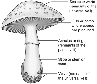
The image below is provided as a visual aid for the reader to recognize different features of a mushroom.
Loading the libraries
import numpy as np
import pandas as pd
pd.set_option('display.float_format', lambda x: '%.5f' % x)
import matplotlib.pyplot as plt
%matplotlib inline
Loading the Data
mushroom_df = pd.read_csv('mushrooms.csv')
Data Exploration
mushroom_df.iloc[:5,:13]
| target | cap-shape | cap-surface | cap-color | bruises | odor | gill-attachment | gill-spacing | gill-size | gill-color | stalk-shape | stalk-root | stalk-surface-above-ring | |
|---|---|---|---|---|---|---|---|---|---|---|---|---|---|
| 0 | edible | convex | smooth | white | bruises | almond | free | crowded | narrow | white | tapering | bulbous | smooth |
| 1 | edible | convex | smooth | white | bruises | almond | free | crowded | narrow | white | tapering | bulbous | smooth |
| 2 | edible | convex | smooth | white | bruises | almond | free | crowded | narrow | pink | tapering | bulbous | smooth |
| 3 | edible | convex | smooth | white | bruises | almond | free | crowded | narrow | pink | tapering | bulbous | smooth |
| 4 | edible | convex | smooth | white | bruises | almond | free | crowded | narrow | brown | tapering | bulbous | smooth |
mushroom_df.iloc[:5,13:]
| stalk-surface-below-ring | stalk-color-above-ring | stalk-color-below-ring | veil-type | veil-color | ring-number | ring-type | spore-print-color | population | habitat | |
|---|---|---|---|---|---|---|---|---|---|---|
| 0 | smooth | white | white | partial | white | one | pendant | purple | several | woods |
| 1 | smooth | white | white | partial | white | one | pendant | brown | several | woods |
| 2 | smooth | white | white | partial | white | one | pendant | purple | several | woods |
| 3 | smooth | white | white | partial | white | one | pendant | brown | several | woods |
| 4 | smooth | white | white | partial | white | one | pendant | purple | several | woods |
print(mushroom_df.info());
RangeIndex: 8416 entries, 0 to 8415
Data columns (total 23 columns):
#   Column                    Non-Null Count  Dtype
---  ------                    --------------  -----
0   target                    8416 non-null   category
1   cap-shape                 8416 non-null   category
2   cap-surface               8416 non-null   category
3   cap-color                 8416 non-null   category
4   bruises                   8416 non-null   category
5   odor                      8416 non-null   category
6   gill-attachment           8416 non-null   category
7   gill-spacing              8416 non-null   category
8   gill-size                 8416 non-null   category
9   gill-color                8416 non-null   category
10  stalk-shape               8416 non-null   category
11  stalk-root                8416 non-null   category
12  stalk-surface-above-ring  8416 non-null   category
13  stalk-surface-below-ring  8416 non-null   category
14  stalk-color-above-ring    8416 non-null   category
15  stalk-color-below-ring    8416 non-null   category
16  veil-type                 8416 non-null   category
17  veil-color                8416 non-null   category
18  ring-number               8416 non-null   category
19  ring-type                 8416 non-null   category
20  spore-print-color         8416 non-null   category
21  population                8416 non-null   category
22  habitat                   8416 non-null   category
dtypes: category(23)
memory usage: 194.1 KB
We start by looking at the datatypes of the feature and output variables.
mushroom_df.dtypes
target                      object
cap-shape                   object
cap-surface                 object
cap-color                   object
bruises                     object
odor                        object
gill-attachment             object
gill-spacing                object
gill-size                   object
gill-color                  object
stalk-shape                 object
stalk-root                  object
stalk-surface-above-ring    object
stalk-surface-below-ring    object
stalk-color-above-ring      object
stalk-color-below-ring      object
veil-type                   object
veil-color                  object
ring-number                 object
ring-type                   object
spore-print-color           object
population                  object
habitat                     object
dtype: object
We first change the type of all columns from object to category.
from pandas.api.types import CategoricalDtype
mushroom_df = mushroom_df.astype("category")
mushroom_df.dtypes
target                      category
cap-shape                   category
cap-surface                 category
cap-color                   category
bruises                     category
odor                        category
gill-attachment             category
gill-spacing                category
gill-size                   category
gill-color                  category
stalk-shape                 category
stalk-root                  category
stalk-surface-above-ring    category
stalk-surface-below-ring    category
stalk-color-above-ring      category
stalk-color-below-ring      category
veil-type                   category
veil-color                  category
ring-number                 category
ring-type                   category
spore-print-color           category
population                  category
habitat                     category
dtype: object
target is the output column and the rest are the features of mushroom.
features = list(mushroom_df.columns[mushroom_df.columns!='target'])
print(features)
['cap-shape', 'cap-surface', 'cap-color', 'bruises', 'odor', 'gill-attachment', 'gill-spacing', 'gill-size',
'gill-color', 'stalk-shape', 'stalk-root', 'stalk-surface-above-ring', 'stalk-surface-below-ring',
'stalk-color-above-ring', 'stalk-color-below-ring', 'veil-type', 'veil-color', 'ring-number', 'ring-type',
'spore-print-color', 'population', 'habitat']
Next, we divide the data into the feature matrix $X$ and outcome vector $y$.
X = mushroom_df[features].values #features
y = mushroom_df['target'].values #target class
Encoding the categorical features
As we noticed, all the features in this dataset are categorical features but machine learning models require all input and output variables to be numeric. There are multiple aproaches to convert categorical variables into numerics such as Ordinal Encoding, One-Hot Encoding, and Dummy Varibale Encoding. For machine-learning applications, it's almost always safer to handle categorical data using One-Hot encoding. We use sklearn's OneHotEncoder in this project.
Let's briefly overview what happens when we One-Hot encode a categorical feature. Let's assume we have a feature column color with colors yellow, blue, and purple.
| index | color |
|---|---|
| 0 | blue |
| 1 | purple |
| 2 | blue |
| 3 | blue |
| 4 | blue |
| 5 | yellow |
| 6 | blue |
| 7 | blue |
| 8 | yellow |
| 9 | blue |
| 10 | purple |
| 11 | purple |
One-Hot encoder encodes each color using using a unique vector length $n$ with $n-1$ $0$s and one $1$ where $n$ is the number of unique colors. The position of $1$ in the vector depends on the color. For example the One-Hot encoded representation of the above example will look like:
| index | color_blue | color_purple | color_yellow |
|---|---|---|---|
| 0 | 1 | 0 | 0 |
| 1 | 0 | 1 | 0 |
| 2 | 1 | 0 | 0 |
| 3 | 1 | 0 | 0 |
| 4 | 1 | 0 | 0 |
| 5 | 0 | 0 | 1 |
| 6 | 1 | 0 | 0 |
| 7 | 1 | 0 | 0 |
| 8 | 0 | 0 | 1 |
| 9 | 1 | 0 | 0 |
| 10 | 0 | 1 | 0 |
| 11 | 0 | 1 | 0 |
Now that we have a basic understanding about encoding the categorical variables into numerics, we can define a function to transform categorical features to One-Hot encoded features.
from sklearn.preprocessing import OneHotEncoder, LabelEncoder
from sklearn.model_selection import train_test_split
# encode the input data
def prepare_inputs(X_train, X_test):
# Set "handle_unknown" argument to "ignore". This is useful in case the model encounters a
# new feature level. Foe example, you train a model with unique colors "blue", "purple", and "yellow"
# and there is a color "red" appearing in the test data.
oh_encoder = OneHotEncoder(handle_unknown="ignore")
oh_encoder.fit(X_train)
X_train_enc = oh_encoder.transform(X_train)
X_test_enc = oh_encoder.transform(X_test)
return X_train_enc, X_test_enc
# encode the target
def prepare_targets(y_train, y_test):
# LableEncoder is pretty much the same as One-Hot encoder but is used for the target variable (labels)
le = LabelEncoder()
le.fit(y_train)
y_train_enc = le.transform(y_train)
y_test_enc = le.transform(y_test)
return y_train_enc, y_test_enc
Splitting the dataset to training (80%) and test data (20%)
X_train, X_test, y_train, y_test = train_test_split(X, y, test_size=0.3, random_state=1)
X_train_enc, X_test_enc = prepare_inputs(X_train, X_test)
y_train_enc, y_test_enc = prepare_targets(y_train, y_test)
The One-Hot encoded features can be obtained using get_feature_names method of the encoder:
oh_encoder_all = OneHotEncoder()
oh_encoder_all.fit(X)
encoded_features = oh_encoder_all.get_feature_names(features)
print(encoded_features)
['cap-shape_bell' 'cap-shape_conical' 'cap-shape_convex' 'cap-shape_flat'
'cap-shape_knobbed' 'cap-shape_sunken' 'cap-surface_fibrous'
'cap-surface_grooves' 'cap-surface_scaly' 'cap-surface_smooth'
'cap-color_brown' 'cap-color_buff' 'cap-color_cinnamon' 'cap-color_gray'
'cap-color_green' 'cap-color_pink' 'cap-color_purple' 'cap-color_red'
'cap-color_white' 'cap-color_yellow' 'bruises_bruises' 'bruises_no'
'odor_almond' 'odor_anise' 'odor_creosote' 'odor_fishy' 'odor_foul'
'odor_musty' 'odor_none' 'odor_pungent' 'odor_spicy'
'gill-attachment_attached' 'gill-attachment_free' 'gill-spacing_close'
'gill-spacing_crowded' 'gill-size_broad' 'gill-size_narrow'
'gill-color_black' 'gill-color_brown' 'gill-color_buff'
'gill-color_chocolate' 'gill-color_gray' 'gill-color_green'
'gill-color_orange' 'gill-color_pink' 'gill-color_purple'
'gill-color_red' 'gill-color_white' 'gill-color_yellow'
'stalk-shape_enlarging' 'stalk-shape_tapering' 'stalk-root_?'
'stalk-root_bulbous' 'stalk-root_club' 'stalk-root_equal'
'stalk-root_rooted' 'stalk-surface-above-ring_fibrous'
'stalk-surface-above-ring_scaly' 'stalk-surface-above-ring_silky'
'stalk-surface-above-ring_smooth' 'stalk-surface-below-ring_fibrous'
'stalk-surface-below-ring_scaly' 'stalk-surface-below-ring_silky'
'stalk-surface-below-ring_smooth' 'stalk-color-above-ring_brown'
'stalk-color-above-ring_buff' 'stalk-color-above-ring_cinnamon'
'stalk-color-above-ring_gray' 'stalk-color-above-ring_orange'
'stalk-color-above-ring_pink' 'stalk-color-above-ring_red'
'stalk-color-above-ring_white' 'stalk-color-above-ring_yellow'
'stalk-color-below-ring_brown' 'stalk-color-below-ring_buff'
'stalk-color-below-ring_cinnamon' 'stalk-color-below-ring_gray'
'stalk-color-below-ring_orange' 'stalk-color-below-ring_pink'
'stalk-color-below-ring_red' 'stalk-color-below-ring_white'
'stalk-color-below-ring_yellow' 'veil-type_partial' 'veil-color_brown'
'veil-color_orange' 'veil-color_white' 'veil-color_yellow'
'ring-number_none' 'ring-number_one' 'ring-number_two'
'ring-type_evanescent' 'ring-type_flaring' 'ring-type_large'
'ring-type_none' 'ring-type_pendant' 'spore-print-color_black'
'spore-print-color_brown' 'spore-print-color_buff'
'spore-print-color_chocolate' 'spore-print-color_green'
'spore-print-color_orange' 'spore-print-color_purple'
'spore-print-color_white' 'spore-print-color_yellow'
'population_abundant' 'population_clustered' 'population_numerous'
'population_scattered' 'population_several' 'population_solitary'
'habitat_grasses' 'habitat_leaves' 'habitat_meadows' 'habitat_paths'
'habitat_urban' 'habitat_waste' 'habitat_woods']
print(f'The dataset has {X.shape[1]} features and {len(encoded_features)} One-Hot encoded features')
The dataset has 22 features and 117 One-Hot encoded features.
Baseline Classifier
We start off with a baseline solution and train a logistic regression classifier. Later, we compare the performance of the decision tree model with the baseline solution and see if we can come up with a decision tree model that surpasses the performance of the baseline solution.
clf_logreg = LogisticRegression(solver='lbfgs')
clf_logreg.fit(X_train_enc, y_train_enc)
y_pred = clf_logreg.predict(X_test_enc)
We can use different metrics to assess the performance of the logistic regression classifier.
from sklearn.metrics import accuracy_score, classification_report
print(classification_report(y_test_enc, y_pred, digits=3))
              precision    recall  f1-score   support
           0      1.000     1.000     1.000      1317
           1      1.000     1.000     1.000      1208
    accuracy                          1.000      2525
   macro avg      1.000     1.000     1.000      2525
weighted avg      1.000     1.000     1.000      2525
accuracy = accuracy_score(y_test_enc, y_pred)
print('Accuracy: %.2f' % (accuracy*100))
Accuracy: 100.00
The baseline classifier reaches perfect accuracy with 100% accuracy! This makes making a more complex solution pointless as the baseline solution is flawless! Let's reduce the number of training samples to make the problem a bit harder for our baseline classifier!
Using a smaller training set: splitting the dataset to training (10%) and test data (90%)!
# We are going to use indices later!
indices = np.arange(len(mushroom_df))
X_train, X_test, y_train, y_test, tr_ids, test_ids = train_test_split(X, y, indices, test_size=0.9, random_state=10)
X_train_enc, X_test_enc = prepare_inputs(X_train, X_test)
y_train_enc, y_test_enc = prepare_targets(y_train, y_test)
clf_logreg = LogisticRegression(solver='lbfgs')
clf_logreg.fit(X_train_enc, y_train_enc)
y_pred = clf_logreg.predict(X_test_enc)
print(classification_report(y_test_enc, y_pred, digits=3))
              precision    recall  f1-score   support
           0      0.996     1.000     0.998      4052
           1      1.000     0.995     0.998      3523
    accuracy                          0.998      7575
   macro avg      0.998     0.998     0.998      7575
weighted avg      0.998     0.998     0.998      7575
from sklearn.metrics import confusion_matrix, ConfusionMatrixDisplay
cm = confusion_matrix(y_test_enc, y_pred)
cm
array([[4052,    0],
      [  16, 3507]])
fig, ax = plt.subplots(1, 1, dpi=120)
cm_plot = ConfusionMatrixDisplay(confusion_matrix=cm, display_labels=['edible', 'poisonous'])
ax.set_title('Logistic regression consfusion matrix')
cm_plot.plot(ax=ax);

Even though we really pushed the limits of the logistic regression classifier by reducing the number of training data, the classifier still does a great job of predicting the correct class. There are, however, 16 instances that the classifier demonstrates type II error by labeling poisonous mushrooms as edible. This is something concerning because in reality this can cause harch consequences. We can now start building the decision tree classifier and see if we can improve the accuracy of the model in identifying poisonous mushrooms compared to the baseline model.
Decision Tree Classifier
In this section we train two decision tree classifiers with the same exact properties except the criterion to assess the quality of a split. One model uses the Gini impurity index whereas the other uses entropy AKA information gain
from sklearn.tree import DecisionTreeClassifier, export_graphviz
import graphviz
# Create Decision Tree classifer object
clf_gini = DecisionTreeClassifier(criterion="gini", random_state=10, max_depth=5, max_leaf_nodes=10)
clf_entropy = DecisionTreeClassifier(criterion="entropy", random_state=10, max_depth=5, max_leaf_nodes=10)
# Train Decision Tree Classifer
clf_gini = clf_gini.fit(X_train_enc,y_train_enc)
clf_entropy = clf_entropy.fit(X_train_enc,y_train_enc)
# Predict the response for test dataset
y_pred_gini = clf_gini.predict(X_test_enc)
y_pred_entropy = clf_entropy.predict(X_test_enc)
y_pred_gini, digits=3))
              precision    recall  f1-score   support
           0      0.996     0.994     0.995      4052
           1      0.993     0.995     0.994      3523
    accuracy                          0.995      7575
   macro avg      0.995     0.995     0.995      7575
weighted avg      0.995     0.995     0.995      7575
print(classification_report(y_test_enc, y_pred_entropy, digits=3))
              precision    recall  f1-score   support
           0      0.998     1.000     0.999      4052
           1      1.000     0.998     0.999      3523
    accuracy                          0.999      7575
   macro avg      0.999     0.999     0.999      7575
weighted avg      0.999     0.999     0.999      7575
fig, ax = plt.subplots(1, 1, dpi=120)
cm = confusion_matrix(y_test_enc, y_pred_gini)
cm_plot = ConfusionMatrixDisplay(confusion_matrix=cm, display_labels=['edible', 'poisonous'])
ax.set_title('Decision tree consfusion matrix')
cm_plot.plot(ax=ax);

fig, ax = plt.subplots(1, 1, dpi=120)
cm = confusion_matrix(y_test_enc, y_pred_entropy)
cm_plot = ConfusionMatrixDisplay(confusion_matrix=cm, display_labels=['edible', 'poisonous'])
ax.set_title('Decision tree consfusion matrix')
cm_plot.plot(ax=ax);
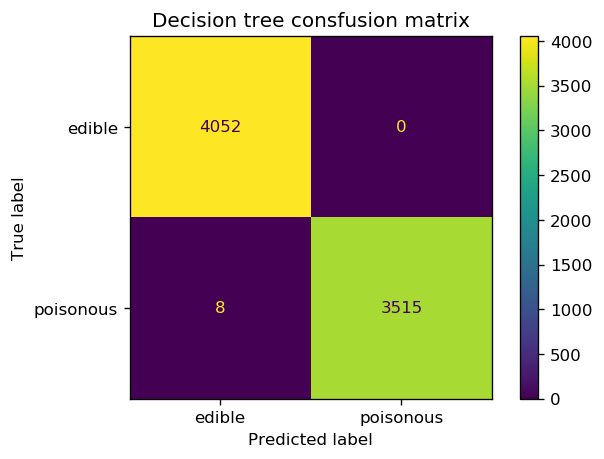
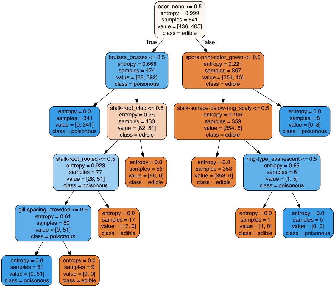
We note that the decision tree with the entropy criterion reaches a higher accuracy than the other tree as well as the baseline classifier. We can generate a plot of the decision tree and look at the rules that the tree has used to defines each split.
from sklearn.tree import export_graphviz
from io import StringIO
from IPython.display import Image
from pydot import graph_from_dot_data
import pydotplus
dot_data = StringIO()
# Training feature names
oh_encoder_tr = OneHotEncoder(handle_unknown="ignore")
oh_encoder_tr.fit(X_train)
encoded_tr_features = oh_encoder_tr.get_feature_names(features)
# Export the tree
export_graphviz(clf_entropy, out_file=dot_data,
filled=True, rounded=True,
special_characters=False,
feature_names = encoded_tr_features,
class_names=['edible', 'poisonous'])
graph = pydotplus.graph_from_dot_data(dot_data.getvalue())
Image(graph.create_png(), width=800, height=400)
Another simple yet useful way to present the decision tree result is using the tree.export_text method of sklearn
from sklearn.tree import export_text
tree_text = export_text(clf_entropy, feature_names = list(encoded_tr_features))
print(tree_text)
|--- odor_none <= 0.50
|   |--- bruises_bruises <= 0.50
|   |   |--- class: 1
|   |--- bruises_bruises >  0.50
|   |   |--- stalk-root_club <= 0.50
|   |   |   |--- stalk-root_rooted <= 0.50
|   |   |   |   |--- gill-spacing_crowded <= 0.50
|   |   |   |   |   |--- class: 1
|   |   |   |   |--- gill-spacing_crowded >  0.50
|   |   |   |   |   |--- class: 0
|   |   |   |--- stalk-root_rooted >  0.50
|   |   |   |   |--- class: 0
|   |   |--- stalk-root_club >  0.50
|   |   |   |--- class: 0
|--- odor_none >  0.50
|   |--- spore-print-color_green <= 0.50
|   |   |--- stalk-surface-below-ring_scaly <= 0.50
|   |   |   |--- class: 0
|   |   |--- stalk-surface-below-ring_scaly >  0.50
|   |   |   |--- ring-type_evanescent <= 0.50
|   |   |   |   |--- class: 0
|   |   |   |--- ring-type_evanescent >  0.50
|   |   |   |   |--- class: 1
|   |--- spore-print-color_green >  0.50
|   |   |--- class: 1
Model diagnosis
One critical step before attempting to improve the accuracy of any model is to figure out what is going wrong. In our case, we would like to see if we can figure out what causes the model giving wrong predictions. First we take a look at the features that are used to train the model and see if there are any features in the test cases that the model has not seen before. This is a common case when dealing with decison tree classifiers with categorical features.
oh_encoder = OneHotEncoder()
oh_encoder.fit(X_test)
encoded_test_features = oh_encoder.get_feature_names(features)
len(encoded_test_features), len(encoded_tr_features)
(117, 113)
We can take a look at the difference between the two lists:
list(encoded_tr_features)))
['cap-shape_conical',
'cap-surface_grooves',
'stalk-color-above-ring_yellow',
'veil-color_yellow']
The model has not seen these features in the training phase. Next, we take a look at the records that have at least one of the above features.
unseen_data = mushroom_df[
    (mushroom_df['cap-shape']=='conical')
  | (mushroom_df['cap-surface']=='grooves')
  | (mushroom_df['veil-color']=='yellow')
  | (mushroom_df['stalk-color-above-ring']=='yellow')
]
unseen_data
| target | cap-shape | cap-surface | cap-color | bruises | odor | gill-attachment | gill-spacing | gill-size | gill-color | ... | stalk-surface-below-ring | stalk-color-above-ring | stalk-color-below-ring | veil-type | veil-color | ring-number | ring-type | spore-print-color | population | habitat | |
|---|---|---|---|---|---|---|---|---|---|---|---|---|---|---|---|---|---|---|---|---|---|
| 6064 | poisonous | bell | grooves | white | bruises | none | free | crowded | narrow | white | ... | smooth | white | white | partial | white | one | pendant | white | clustered | leaves |
| 6066 | poisonous | conical | grooves | white | bruises | none | free | crowded | narrow | white | ... | smooth | white | white | partial | white | one | pendant | white | clustered | leaves |
| 6067 | poisonous | conical | scaly | white | bruises | none | free | crowded | narrow | white | ... | smooth | white | white | partial | white | one | pendant | white | clustered | leaves |
| 6068 | poisonous | flat | grooves | white | bruises | none | free | crowded | narrow | white | ... | smooth | white | white | partial | white | one | pendant | white | clustered | leaves |
| 6070 | poisonous | knobbed | grooves | white | bruises | none | free | crowded | narrow | white | ... | smooth | white | white | partial | white | one | pendant | white | clustered | leaves |
| 7880 | poisonous | bell | scaly | yellow | no | none | free | crowded | narrow | yellow | ... | scaly | yellow | yellow | partial | yellow | one | evanescent | white | clustered | leaves |
| 7881 | poisonous | bell | scaly | yellow | no | none | free | crowded | narrow | white | ... | scaly | yellow | yellow | partial | yellow | one | evanescent | white | clustered | leaves |
| 7882 | poisonous | conical | scaly | yellow | no | none | free | crowded | narrow | yellow | ... | scaly | yellow | yellow | partial | yellow | one | evanescent | white | clustered | leaves |
| 7883 | poisonous | conical | scaly | yellow | no | none | free | crowded | narrow | white | ... | scaly | yellow | yellow | partial | yellow | one | evanescent | white | clustered | leaves |
| 7884 | poisonous | flat | scaly | yellow | no | none | free | crowded | narrow | yellow | ... | scaly | yellow | yellow | partial | yellow | one | evanescent | white | clustered | leaves |
| 7885 | poisonous | flat | scaly | yellow | no | none | free | crowded | narrow | white | ... | scaly | yellow | yellow | partial | yellow | one | evanescent | white | clustered | leaves |
| 7886 | poisonous | knobbed | scaly | yellow | no | none | free | crowded | narrow | yellow | ... | scaly | yellow | yellow | partial | yellow | one | evanescent | white | clustered | leaves |
| 7887 | poisonous | knobbed | scaly | yellow | no | none | free | crowded | narrow | white | ... | scaly | yellow | yellow | partial | yellow | one | evanescent | white | clustered | leaves |
13 rows × 23 columns
X_test_unseen = unseen_data[features].values
__, X_test_unseen_enc = prepare_inputs(X_train, X_test_unseen)
y_pred_unseen = clf_entropy.predict(X_test_unseen_enc)
y_pred_unseen
array([0, 0, 0, 0, 0, 1, 1, 1, 1, 1, 1, 1, 1])
We notice that 5 out of the 8 wrong predictoins belong to the instances with features that the model has not seen during the training phase. All the wrong predictions can be found using:
false_predictions = np.where(y_test_enc!=y_pred_entropy)
false_predictions
(array([3535, 4237, 4628, 4734, 5692, 6063, 7159, 7283]),)
np.sort(test_ids[false_predictions])
array([6064, 6065, 6066, 6067, 6068, 6069, 6070, 6071])
Now we can take a closer look at the recoreds that were misclassified by the tree:
mushroom_df.iloc[np.sort(test_ids[false_predictions]), :12]
| target | cap-shape | cap-surface | cap-color | bruises | odor | gill-attachment | gill-spacing | gill-size | gill-color | stalk-shape | stalk-root | |
|---|---|---|---|---|---|---|---|---|---|---|---|---|
| 6064 | poisonous | bell | grooves | white | bruises | none | free | crowded | narrow | white | enlarging | bulbous |
| 6065 | poisonous | bell | scaly | white | bruises | none | free | crowded | narrow | white | enlarging | bulbous |
| 6066 | poisonous | conical | grooves | white | bruises | none | free | crowded | narrow | white | enlarging | bulbous |
| 6067 | poisonous | conical | scaly | white | bruises | none | free | crowded | narrow | white | enlarging | bulbous |
| 6068 | poisonous | flat | grooves | white | bruises | none | free | crowded | narrow | white | enlarging | bulbous |
| 6069 | poisonous | flat | scaly | white | bruises | none | free | crowded | narrow | white | enlarging | bulbous |
| 6070 | poisonous | knobbed | grooves | white | bruises | none | free | crowded | narrow | white | enlarging | bulbous |
| 6071 | poisonous | knobbed | scaly | white | bruises | none | free | crowded | narrow | white | enlarging | bulbous |
Interestingly, a little bit of investigation shows that the misclassified instances can be found using the following rules:
mushroom_df[
    (mushroom_df['cap-color']=='white')
  & (mushroom_df['bruises']=='bruises')
  & (mushroom_df['odor']=='none')
  & (mushroom_df['gill-spacing']=='crowded')
]
| target | cap-shape | cap-surface | cap-color | bruises | odor | gill-attachment | gill-spacing | gill-size | gill-color | ... | stalk-surface-below-ring | stalk-color-above-ring | stalk-color-below-ring | veil-type | veil-color | ring-number | ring-type | spore-print-color | population | habitat | |
|---|---|---|---|---|---|---|---|---|---|---|---|---|---|---|---|---|---|---|---|---|---|
| 6064 | poisonous | bell | grooves | white | bruises | none | free | crowded | narrow | white | ... | smooth | white | white | partial | white | one | pendant | white | clustered | leaves |
| 6065 | poisonous | bell | scaly | white | bruises | none | free | crowded | narrow | white | ... | smooth | white | white | partial | white | one | pendant | white | clustered | leaves |
| 6066 | poisonous | conical | grooves | white | bruises | none | free | crowded | narrow | white | ... | smooth | white | white | partial | white | one | pendant | white | clustered | leaves |
| 6067 | poisonous | conical | scaly | white | bruises | none | free | crowded | narrow | white | ... | smooth | white | white | partial | white | one | pendant | white | clustered | leaves |
| 6068 | poisonous | flat | grooves | white | bruises | none | free | crowded | narrow | white | ... | smooth | white | white | partial | white | one | pendant | white | clustered | leaves |
| 6069 | poisonous | flat | scaly | white | bruises | none | free | crowded | narrow | white | ... | smooth | white | white | partial | white | one | pendant | white | clustered | leaves |
| 6070 | poisonous | knobbed | grooves | white | bruises | none | free | crowded | narrow | white | ... | smooth | white | white | partial | white | one | pendant | white | clustered | leaves |
| 6071 | poisonous | knobbed | scaly | white | bruises | none | free | crowded | narrow | white | ... | smooth | white | white | partial | white | one | pendant | white | clustered | leaves |
8 rows × 23 columns
But the model has not encountered this situation during the training as seen below:
mushroom_df_tr = mushroom_df.iloc[np.sort(tr_ids), :]
mushroom_df_tr[
    (mushroom_df_tr['cap-color']=='white')
  & (mushroom_df_tr['bruises']=='bruises')
  & (mushroom_df_tr['odor']=='none')
  & (mushroom_df_tr['gill-spacing']=='crowded')
]
| target | cap-shape | cap-surface | cap-color | bruises | odor | gill-attachment | gill-spacing | gill-size | gill-color | ... | stalk-surface-below-ring | stalk-color-above-ring | stalk-color-below-ring | veil-type | veil-color | ring-number | ring-type | spore-print-color | population | habitat |
|---|
0 rows × 23 columns
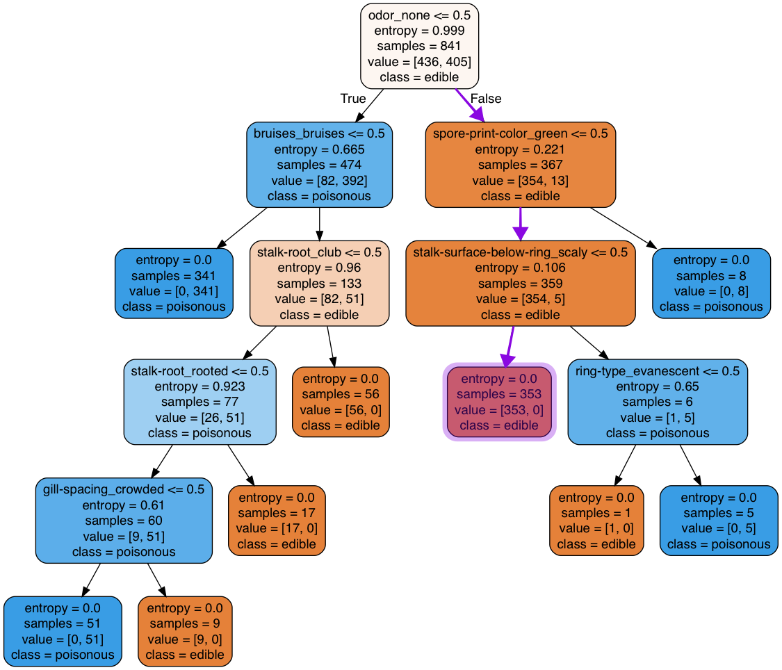
We can investigate what caused these wrong predictions by considering the featutes that are common between the misclassified instances and walk down the tree to see at which split the misclassification occurs. odor=none, meaning that odor_none$\leq$0.5 is False (because odor_none=1) so in the first split on the tree we move to the right) spore-print-color=white, meaning that spore-print-color_green$\leq$0.5 is True so in the next split on the tree we move to the left stalk-surface-below-ring=smooth, meaning that stalk-surface-below-ring_scaly$\leq$0.5 is True so in the next split on the tree we move to the left. At this point, we have reached a leaf that according to the trained model gives the output for the misclassifies instances to be edible. The process is shown using a purple arrow in the figure below.
Note that what this means is no matter how much we change the tree structure (increase the tree depth, leaf nodes, etc.), the misclassified instances will remain misclassified! In other words, increasing the complexity of the tree is not a solution. We can, however, find a tree with the same exact strucure as the current tree by traying different training-set samplings. We would also test the baseline estimator on these instances for the sake of comparison.
Cross-validation
Here we use cross-validation by re-sampling the training-data 10 times while conserving the size of training set.
num_val_tests = 20
best_tree_model = clf_entropy
best_tree_score = best_tree_model.score(X_test_enc, y_test_enc)
best_logreg_model = clf_logreg
best_logreg_score = best_logreg_model.score(X_test_enc, y_test_enc)
for i in range(num_val_tests):
    seed = np.random.randint(1000)
    # train/test split
    X_train, X_test, y_train, y_test, tr_ids, test_ids = train_test_split(
        X, y, indices, test_size=0.9, random_state=seed
    )
    # instantiate the DecisionTreeClassifier and the
    clf_tree_tmp = DecisionTreeClassifier(
        criterion="entropy", random_state=10, max_depth=5, max_leaf_nodes=10
    )
    clf_logreg_tmp = LogisticRegression(solver='lbfgs')
    # encode train/test
    X_train_enc, X_test_enc = prepare_inputs(X_train, X_test)
    y_train_enc, y_test_enc = prepare_targets(y_train, y_test)
    # fit
    clf_tree_tmp = clf_tree_tmp.fit(X_train_enc,y_train_enc)
    clf_logreg_tmp = clf_logreg_tmp.fit(X_train_enc,y_train_enc)
    # evaluate
    tree_score = clf_tree_tmp.score(X_test_enc, y_test_enc)
    logreg_score = clf_logreg_tmp.score(X_test_enc, y_test_enc)
    # compare with the best tree model so far
    if tree_score > best_tree_score:
        best_tree_score = tree_score
        best_tree_model = clf_tree_tmp
        X_enc_best_tree = X_test_enc
        y_enc_best_tree = y_test_enc
        seed_best_tree = seed
    # repeat for the logistic regression model
    if logreg_score > best_logreg_score:
        best_logreg_score = logreg_score
        best_logreg_model = clf_logreg_tmp
        X_enc_best_logreg = X_test_enc
        y_enc_best_logreg = y_test_enc
        seed_best_logreg = seed
print(f"best decision tree model reaches the accuracy {np.round(best_tree_score*100, 3)}%")
print(f"best logistic regression model reaches the accuracy {np.round(best_logreg_score*100, 3)}%")
best decision tree model reaches the accuracy 100.0%
best logistic regression model reaches the accuracy 99.908%
We note that without having to increase the complexity of the model, we were able to find a perfect model.
y_pred_tree = best_tree_model.predict(X_enc_best_tree)
y_pred_logreg = best_logreg_model.predict(X_enc_best_logreg)
print(classification_report(y_enc_best_tree, y_pred_tree, digits=3))
              precision    recall  f1-score   support
           0      1.000     1.000     1.000      4015
           1      1.000     1.000     1.000      3560
    accuracy                          1.000      7575
   macro avg      1.000     1.000     1.000      7575
weighted avg      1.000     1.000     1.000      7575
fig, ax = plt.subplots(1, 1, dpi=120)
cm = confusion_matrix(y_enc_best_tree, y_pred_tree)
cm_plot = ConfusionMatrixDisplay(confusion_matrix=cm, display_labels=['edible', 'poisonous'])
ax.set_title('Decision tree consfusion matrix')
cm_plot.plot(ax=ax);

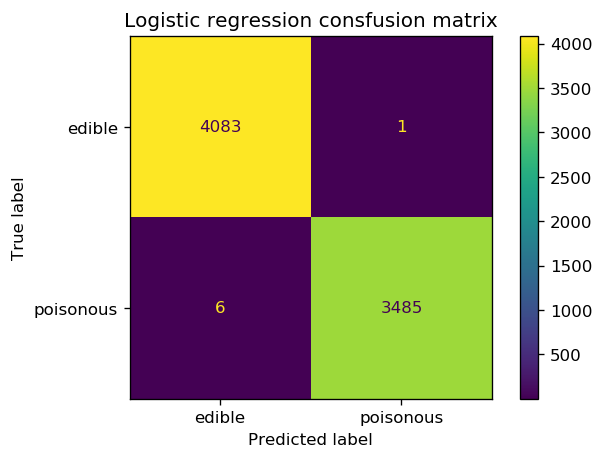
print(classification_report(y_enc_best_logreg, y_pred_logreg, digits=3))
              precision    recall  f1-score   support
           0      0.999     1.000     0.999      4084
           1      1.000     0.998     0.999      3491
    accuracy                          0.999      7575
   macro avg      0.999     0.999     0.999      7575
weighted avg      0.999     0.999     0.999      7575
fig, ax = plt.subplots(1, 1, dpi=120)
cm = confusion_matrix(y_enc_best_logreg, y_pred_logreg)
cm_plot = ConfusionMatrixDisplay(confusion_matrix=cm, display_labels=['edible', 'poisonous'])
ax.set_title('Logistic regression consfusion matrix')
cm_plot.plot(ax=ax);
Visualizing the best tree
dot_data = StringIO()
# Training feature names
oh_encoder_tr = OneHotEncoder(handle_unknown="ignore")
X_train, X_test, y_train, y_test, tr_ids, test_ids = train_test_split(
    X, y, indices, test_size=0.9, random_state=seed_best_tree
)
oh_encoder_tr.fit(X_train)
encoded_tr_features = oh_encoder_tr.get_feature_names(features)
# Export the tree
export_graphviz(best_tree_model, out_file=dot_data,
                filled=True, rounded=True,
                special_characters=False,
                feature_names = encoded_tr_features,
                class_names=['edible', 'poisonous'])
graph = pydotplus.graph_from_dot_data(dot_data.getvalue())
Image(graph.create_png(), width=800, height=400)
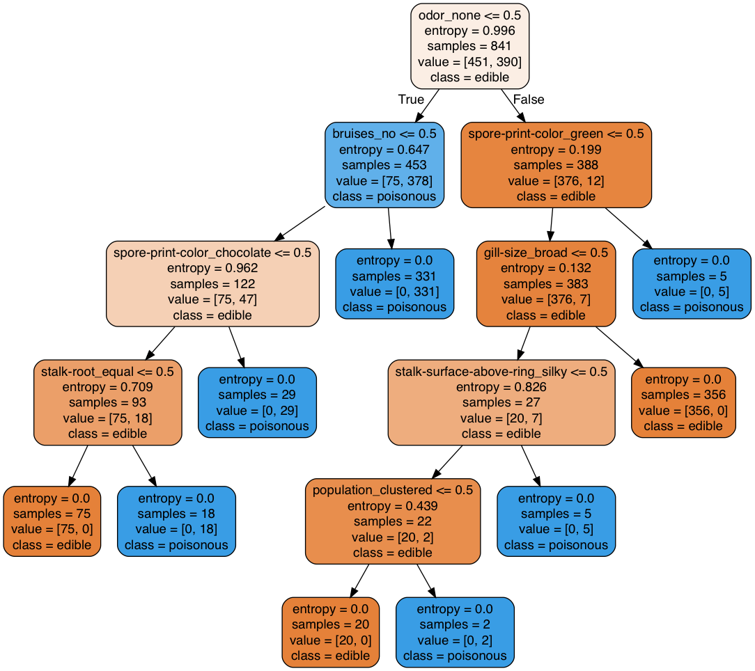
Note that the features that the best tree is using to split on are very different from the ones that were used previously as they depend on the training set that is used to train the tree.
Conslusion
- In this post we applied a decision tree classifier to detect poisonous mushrooms in a mushroom dataset with 8416 records.
- We learned that decision tree classifiers can handle unknown features in the test set but these unknown features are likely to be misclassified
- We lobserved that there are certain situations that the error is due to lack of training data and the only way to resolve the misclassified instances is to train the model using new data. We achieved this by cross-validation.
- Cross-validation is a great asset to keep the model simple and prevent overfitting.
- We noticed that diagnosing the model before attempting to increase the complexity of the model can sometimes be beneficial and lead to a model with a better accuracy without necessarily adding to the complexity of the model